CityFloodMap.com reaches 500,000 views - thank you!

 Hi all,

Thank you so much for your interest in CityFloodMap.com and the material that I post. We have just surpassed half a million views!

I started this blog in 2013 when many of the topics covered were popping up at work and I realized that they deserved a "deep dive". As the very first post says:

"Welcome to the Urban Flooding blog.

The blog is intended to support discussion on urban flooding issues and solutions.  It will share information on urban flood risk management through long term strategies including risk identification, prioritization and prevention.

Rob"

That explains the 'Why?" of this blog, to better characterize urban flooding and how we should best address it. The need for this material is now as important as ever as the Canadian government develops and advances its climate change adaptation strategy.

I'd like to thank a few people for putting me on the right track. That includes Dr. Barry Adams, my Master thesis supervisor (and the reason I switched from structural engineering to water resources during my undergrad degree). I had reached out to Dr. Adams following my earliest reviews of extreme rainfall trends, asking if he also saw the disconnect occurring in the media, and even in the engineering community - how come the facts and data on extreme rainfall were not being openly acknowledged? My concern was that residents in the community where I work  (and also senior staff and decision/policy makers) were being misguided and that could adversely affect the direction of adaptation initiatives for flood control. Dr. Adams encouraged me to publish some of my findings and that ultimately that led to the paper "Evidence Based Policy Gaps in Water Resources: Thinking Fast and Slow on Floods and Flow" in the Journal of Water Management Modeling (https://www.chijournal.org/C449).

Others I'd like to thank include our previous MPP Arthur Potts (https://en.wikipedia.org/wiki/Arthur_Potts_(politician)). I met with MPP Potts early on suggesting that the province of Ontario needed to be better aware of extreme rainfall trends and the drivers affecting infrastructure investment priorities. MPP Potts suggested that advancing these ideas would be most-effectively be made through professional, industry organizations to provide a stronger voice what could help shape policies and standards. With that began my work with Ontario's Municipal Engineers Association and its Ministry of the Environment liaison committee, the Water Environment Association of Ontario and its Collection Systems and Government Affairs committees, and the Ontario Society of Professional Engineers and its Infrastructure Task Force. These have proven to be effective avenues for sharing technical information that can shape policies and priorities reflected in legislation, guidelines and standards.

Dr. Adams also helped make connections with others who shared an interest in advancing ideas in this blog connecting me with Fabian Papa, a University of Toronto alumnus and founding partner of fabian papa & partners (https://www.fabianpapa.com/) and a principal of HydraTek & Associates. Together we have been advancing many of the ideas in this blog through several channels: a white paper on policy gaps for the National Research Council of Canada, peer review of risk research for a local Conservation Authority, presentations at technical workshops, regional and national conferences (WEAO, CWWA), magazine articles (WEAO Influents) and most recently the development of the National Research Council of Canada's flood control cost benefit guidelines (https://nrc-publications.canada.ca/eng/view/object/?id=27058e87-e928-4151-8946-b9e08b44d8f7).   

Some people in the insurance industry have also been interested in the material on this blog. I was invited by Insurance Business Magazine to present at their 2016 Flood Master Class (https://www.slideshare.net/RobertMuir3/flood-plains-to-floor-drains-design-standard-adaptation-for-urban-flood-risk-reduction) - my presentation "Flood plains to floor drains design standard adaptation for urban flood risk reduction" spoke to factors other than changes in extreme rainfall affecting flood risks, and the role of historical standards for storm drainage, wastewater collection and floodplain management driving flood risks and adaptation needs.

One insurance industry practitioner had reached out to me based on the mapping of 'lost rivers' to confirm that flood claims in Toronto during the extreme July 8, 2013 event were correlated to my estimated overland flood hazard areas. Others, including third parties providing flood risk information to the insurance industry, have been generous in sharing their estimated riverine and urban/pluvial hazard and damage mapping estimates, and risk scores based on historical claims. This has all help shape the research and findings in the blog and beyond (e.g., as part of consulting assignments), supporting the focus on other evidence-based risk factors beyond extreme rainfall trends. 

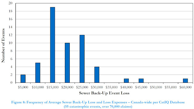
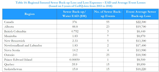
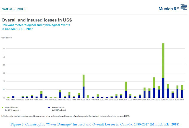
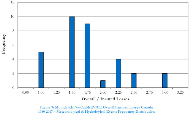
Through a connection Fabian made with the former Environmental Commissioner of Ontario, and as a follow-up to a presentation we made to her office, the insurance industry also shared detailed loss data to support Ontario trend analysis. Similar information was also shared for other regions to support the National Research Council of Canada's flood control cost benefit guideline development - thanks IBC! Some interesting take-aways in the guidelines using industry data were summarized in this blog post: https://www.cityfloodmap.com/2022/02/nrc-national-guidelines-on-flood_27.html. Thanks also to Munich Re for custom Canadian data provided and CatIQ for letting us showcase some of their insightful loss and claim data.

Through this blog I was able to support researchers developing seed documents for national standards - this post "Reducing Flood Risk from Flood Plain to Floor Drain, Developing a Canadian Standard for Design Standard Adaptation in Existing Communities" (https://www.cityfloodmap.com/2018/02/reducing-flood-risk-from-flood-plain-to.html) was foundational research for the Intact Centre on Climate Adaptation's 2019 seed document "Weathering the Storm: Developing a Canadian Standard for Flood-Resilient Existing Communities" (https://www.intactcentreclimateadaptation.ca/wp-content/uploads/2019/01/Weathering-the-Storm.pdf). Subsequently I was on the Canadian Standard's Association's technical subcommittee advancing the standard based on the seed document and called "CSA W210:21, Prioritization of flood risk in existing communities" (https://www.csagroup.org/store/product/2705176/).

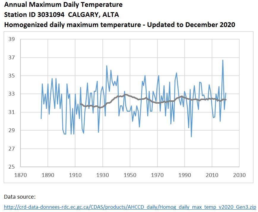
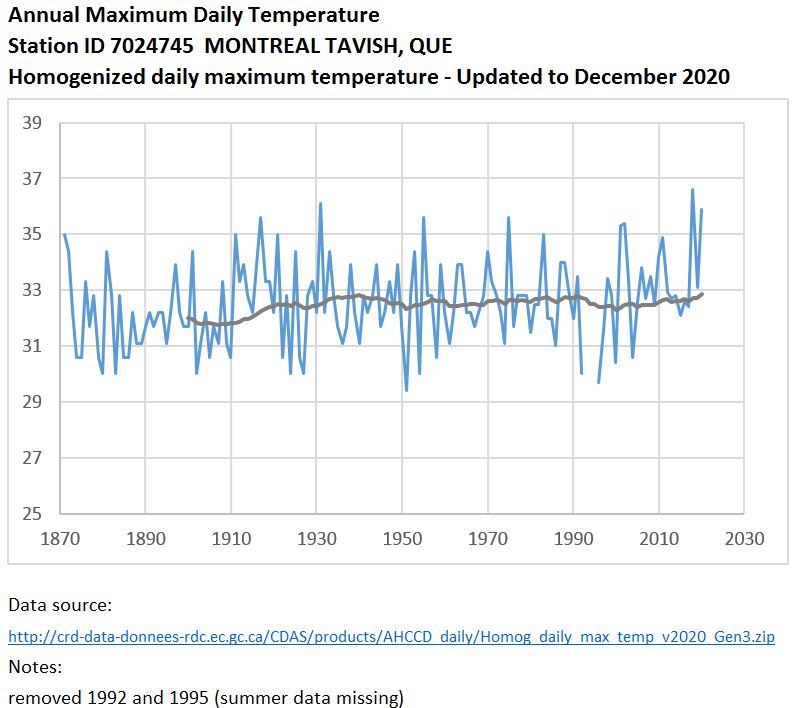
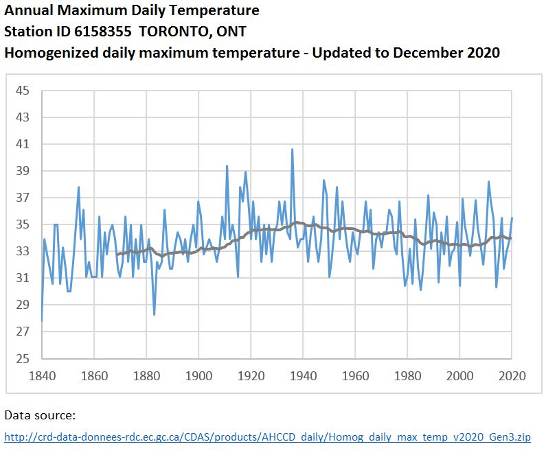
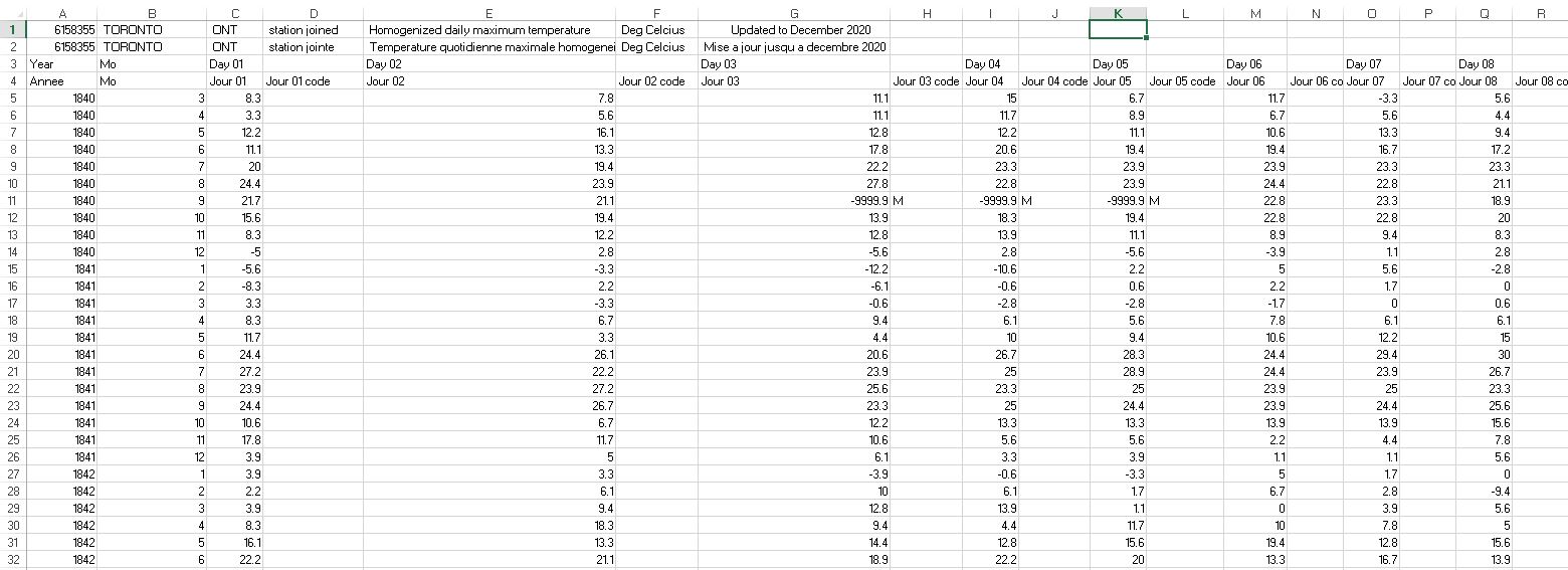
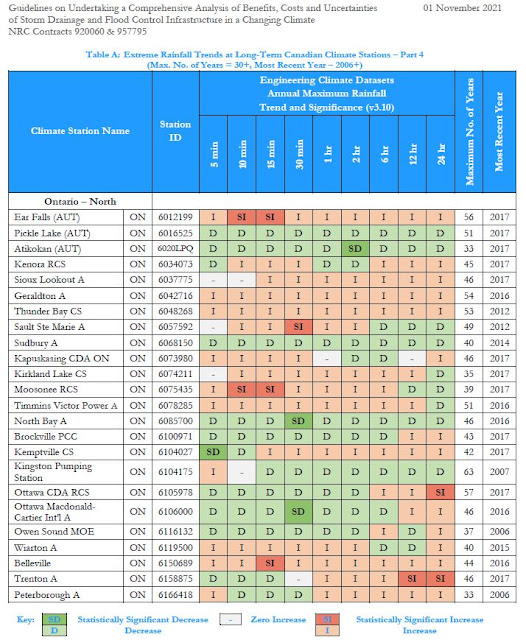
Of course it has been a lot of work - but most of all it has been interesting and worthwhile research that has led to very rewarding connections and accomplishments in guiding risk identification, prioritization and prevention. It has been great to see earlier findings in the "Evidence Based Policy Gaps in Water Resources: Thinking Fast and Slow on Floods and Flow" paper on normalized insurance loss trends later reflected in the Canada in a Changing Climate: National Issues report in 2021 - it shows losses increasing primarily due to growth, not climate effects. Having that paper's earlier findings on extreme rainfall intensity trends in Ontario expanded across Canada and published in the NRC cost benefit guidelines was a worthwhile as well - those trends help define risk drivers and guide the most effective adaptation solutions.

Material in this blog has helped frame discussions in the media and improve the accuracy of reporting on extreme weather trends and risks too. Editors and the Ombudsman offices at Radio-Canada and CBC have corrected or even deleted inaccurate reporting on that topic over the last several years - several examples are summarized here: https://www.cityfloodmap.com/2019/06/cbc-correcting-claims-on-extreme.html. Why this is important can be seen in this presentation that shows how arbitrary theoretical shifts in extreme weather have been mistakenly described as actual changes in federal data sets: https://www.slideshare.net/RobertMuir3/storm-intensity-not-increasing-factual-review-of-engineering-datasets. The presentation "Storm Intensity Not Increasing. Review of Weather Event Statement in Insurance Bureau of Canada’s “Telling the Weather Story” prepared by Institute for Catastrophic Loss Reduction." shows this quite clearly.

Some media have been effective partners at spreading more accurate perspectives on flood risks founded on data and promoted on this blog - for example Financial Post published an article by me and Dr. Bryan Karney entitled "Fast flood science needs slow thinking Junk Science Week: Media stories on rain and floods bungle the science" (https://financialpost.com/opinion/fast-flood-science-needs-slow-thinking).

In recent years other keen practitioners including former colleagues from across the country have collaborated to promote a better understanding of the design factors affecting risk and resilience in storm drainage systems, as in the technical publication "Toward More Resilient Urban Stormwater Management Systems—Bridging the Gap From Theory to Implementation" (https://www.frontiersin.org/articles/10.3389/frwa.2021.671059/full). A current colleagues has also collaborated on conference papers and presentations to better characterize design considerations affecting risks in wastewater collection systems, including at local WEAO workshops and conferences (e.g., see "Wastewater Collection System Performance Under Climate Change – Safety Factors and Stress Tests for Flood Risk Mitigation", paper: https://drive.google.com/drive/folders/1rB87RHti_XiYHWV-5XeBvBXMq1MVMD0Z?usp=sharing, presentation: https://www.slideshare.net/RobertMuir3/wastewater-collection-system-performance-under-climate-change-safety-factors-and-stress-tests-for-flood-risk-mitigation). These collaborative efforts help advance the fundamental goal of the blog.

That's where I've been. There is some more to come. I led the drafting of Natural Resources Canada's federal flood mapping guideline series on risk prioritization ("Flood Hazard Identification and Priority Setting") a couple years ago. That guideline, once finalized and released could also guide in the screening of flood risks to support further detailed analysis of hazards, damages and prioritization of adaptation needs. I'll be sure to cover any highlights here.

Thank you for reading the blog, and thank you to those who have supported all the related research, and standards and policy advocacy.

Robert Muir

June 5, 2022

Maximum Temperature Trends in Select Canadian Cities - Long-Term Trends from Environment and Climate Change Canada's AHCCD Dataset

A previous post reviewed Environment and Climate Change Canada's Adjusted Homogenized Canadian Climate Data (AHCCD) and temperature trends in Toronto and Ottawa. See post: https://www.cityfloodmap.com/2017/11/tvo-articles-on-climate-change-extreme.html

Temperature changes have been related to extreme rainfall changes, given the higher water holding capacity of warmer air.

This post presents more trends in annual maximum daily temperature at 12 cities across Canada. The AHCCD has recently been updated in 2020 - see summary here: https://www.canada.ca/en/environment-climate-change/services/climate-change/science-research-data/climate-trends-variability/adjusted-homogenized-canadian-data/surface-air-temperature.html

The following charts present the annual maximum temperatures (blue line) and 30-year moving average trends (grey line). Years with missing summer data have been removed. The selection of stations is based on those with long records but is not exhaustive. It is not clear if urban heat island effects could be a factor at these stations as well.

In Calgary the period up to the 1940's and 1950's was warmer (had higher maximum daily temperatures) that the most recent period:

In Chilliwack, temperatures have been fairly steady up until the periods ending in the 2000's after which some very high extremes have occurred:

In Fredericton the 30-year rolling average of maximum daily temperature has been increasing since the period ending in the 1930's, but has been decreasing since about 2000:

In Halifax, the average maximum temperatures here highest in the periods before about 1960, after which there was a drop. Since that drop the average has been increasing since 1990:

In Moncton, the average maximum temperatures have been relatively flat:

In Montreal, pre-1910 had lower daily maximum temperatures on average. Since the 1930's average maximum temperatures have been flat:

In Ottawa, the 30-year average has been decreasing since the late 1800's and early 1900's:

In Saskatoon, the 30-year average of maximum temperatures increased up to1940 and has been decreasing since then:

In St. John's, the daily maximum temperatures decreased in the late 1800's but overall have since been increasing, with a slight recent decrease:

In Vancouver, there appears to be a discontinuity in the data, with no trend up to 1930, a steep increase up to 1960, and generally flat (slightly increasing) trend since then:

Ross McKitrick, Department of Economics and Finance, University of Guelph, has commented on Vancouver temperature trends in the past (see July 2019 article in the Vancouver Sun - link: https://vancouversun.com/opinion/op-ed/ross-mckitrick-reality-check-there-is-no-climate-emergency-in-vancouver). He wrote:

"Temperature records for Vancouver begin in 1896. Looking at the 100 years from 1918 to 2018, February and September average daytime highs rose slightly, at about 1.5 degrees per century, while the other 10 months did not exhibit a statistically significant trend. Looking at the interval from 1938 forward, no month exhibits a significant upward trend in average daytime highs, in fact four months went down slightly. Looking at 1958 to the present, four months warmed slightly, but the annual average daytime high did not exhibit a significant trend." - the chart above supports this observation with annual maximum temperatures 'flat' since the late 1930's.

In Winnipeg, average maximum temperatures have been decreasing since the period ending in about 1950:

In Toronto, the trend is similar to Winnipeg - there were increases up to the periods ending in about the mid 1930's then a decrease: 

The previous post, based on data up to 2018, showed the trends in July daily maximum temperatures for other southern Ontario climate stations including Welland, Vineland, Hamlton, Belleville, Toronto and Peterborough. The trends included increases and decreases and an average increase of 0.17 degrees Celsius at these 6 stations:

 

Additional reading: Ross McKitrick has done a more thorough analysis of Canadian temperatures in his paper "Trends in Historical Daytime Highs in Canada 1888-2017" in 2018 (link: https://www.rossmckitrick.com/uploads/4/8/0/8/4808045/temp_report.pdf). He noted trends across Canada similar to those for southern Ontario above, writing "Since 1939 there has been virtually no change in the median July and August daytime highs across Canada, and October has cooled slightly."

Previous posts explored whether extreme rainfall intensities have increased in Canada - recent updates in Engineering Climate Datasets show no recent increase in 100-year design intensities and longer-term trends in southern Ontario stations have not shown increases in those extremes overall. It is possible that the lack of consistent increases in extreme temperature could be related to the trends in extreme rainfall - of course the charts above are limited to annual maximum daily temperatures and not longer-period temperatures that could also be influencing design rainfall intensities. 

***

How do you analyze temperature data in the AHCCD? 

Some manipulation of the raw AHCCD information is needed to determine annual maximum temperatures and to assess the 30-year trends charted above. The AHCCD data is provided in a compressed 'zip' file that contains individual files for each location, or climate station. Individual files are text files in ASCII format and are named after the climate station ID #. For example Toronto's station ID 6158355 has a data file called dx6158355.txt that looks like this:

This data file can be imported into an MS Excel worksheet and then be parsed, converting long text strings in column A to separate columns (use Text to Column function). Parsed data, with a column title added to the "data code" column after each day's maximum daily temperature data, would look like this:

Each row of data starting on Row 5 above represents the daily maximum temperatures in a single month. The maximum temperatures for each month can be calculated in column BN using the MAX function. For example, the red text shows maximum temperatures in each month (the maximum daily temperature across the row):

To determine the maximum temperature each year, the Excel Pivot Table function can be used. After selecting the column heading Row 4 and all data rows below and Columns A to BN, insert Pivot Table on a new worksheet. In the Pivot Table Fields window, drag "Annee" (year) into the Rows box and drag "Daily_max" into the Values box. The Values field will by default assign a sum function showing "Sum of Daily_max", summing all the monthly maximum temperatures in each year -  change that to a max function by clicking on the field and setting value field setting to "Max":

The result of the Pivot Table is shown below, with the maximum daily temperature determined for each year:

The annual maximum temperatures can be charted using an XY scatter plot in Excel. To create the 30-year moving average trend, insert a trendline (right click on the plotted line and select "Add a trendline").  Change the trendline type of moving average, specifying "Period" of 30 to average 30 years of annual maximum values (i.e., the overall maximum temperature climate trend for the prior 30 years). 

***

Extreme heat and trends can also be characterized using other statistics besides annual maximum temperatures reviewed above. For example, the number of days over a threshold value, such as 30 degrees Celsius, and that would be associated with stresses can be used as well.

The AHCCD data assessed above can be used to count the number of days in each month reaching over a threshold temperature, and those monthly counts can be summed for each year in the record. The example charts below show the number of days in each year with maximum temperature over 30 degrees Celsius. These charts also show the 30-year moving average of number of days over 30 degrees.

In Toronto, the average number of days over 30 degrees was highest many decades ago. The dashed black line shows this average and the ECCC AHCCD data shows that in the 30 years up to 1959 there were 14.9 days above 30 degrees, while in the 30 years up to 2020 there were fewer at 14.0 days a year. In the periods up to 1938-1941 the average number of extremely hot days was also high than the recent past, with 14.4 days above 30 degrees for those earlier periods: 

In Calgary, similar analysis shows that earlier periods were hottest. The 30 year average up to 2020 has an average number of days above 30 degrees of 4.8, compared to the period up to 1941 that had 6.1 days. The recent average of 4.8 days was exceeded in all the periods up to 1933 to 1955, and the periods up to 1986 to 1989 as well: 

Southern Ontario Extreme Rainfall Trends and Engineering Design Considerations for Effective Management

This blog has many posts that illustrate how the media, some researchers, and/or the insurance industry have missed the mark when it comes to defining past changes in extreme rainfall and the effects on communities. What is also apparent is that government agencies and ministries have also missed the mark when it comes to defining these changes and what it means to stormwater management policies and design standards. 

This post provides:

1) Examples of media, researcher and insurance industry data gaps on extreme rainfall compiled over the years;

2) A presentation made to the the Ontario Ministry of the Environment, Conservation and Parks with information for Ontario (MECP) showing inaccurate government statements on past trends, and actual data characterizing southern Ontario trends to help guide development of standards for stormwater systems; and

3) References to updated material that expand on and confirm the above.

***

1) Examples of the media, researchers, and the insurance industry misstating extreme weather and rainfall trends

CBC and Radio-Canada - this blog post compiles corrections by CBC and Radio-Canada related to extreme rainfall frequency since 2015, including corrections to or the deletion of articles that violated their journalistic standards and practices, including the commitment for accuracy in reporting: https://www.cityfloodmap.com/2019/06/cbc-correcting-claims-on-extreme.html

Key take-away: even large media organizations are not well-equipped to critically report on the basics of extreme rainfall. 

TVO - this blog post includes a critique of storm intensity and extreme temperature reporting in 2017 and 2019: https://www.cityfloodmap.com/2017/11/tvo-articles-on-climate-change-extreme.html

Key take-away: smaller media organizations are not well-equipped to critically report on the basics of extreme rainfall or temperature trends either. 

Insurance Industry / Researchers (plus more media) - this presentation shows that many cannot tell the difference between a theoretical, arbitrary 'bell-curve' shift in extreme weather frequency and actual observations, and that there is no fact-checking in most media. This relates to the widely-reported incorrect claim in the Institute for Catastrophic Loss Reduction (ICLR) report "Telling the Weather Story" for the Insurance Bureau of Canada (IBC) that "weather events that used to happen once every 40 years are now happening once every size years": https://www.slideshare.net/RobertMuir3/storm-intensity-not-increasing-factual-review-of-engineering-datasets

Key take-away: media organizations, and even the chief economist at a large Canadian bank, do not verify suggested extreme rainfall or weather trends in Canada, and will widely echo unsupported/incorrect/false statements. In this case the insurance industry had not checked the researcher statements in a report they commissioned.

2) MECP presentation on extreme rainfall trends to guide stormwater design standards

The MECP embanked on the development of design standards for wastewater and stormwater systems in Ontario to support Consolidated Linear Infrastructure (CLI) Environmental Compliance Approvals (ECAs). CLI ECA's for stormwater systems (like wastewater systems) are intended to consolidate individual ECA's for stormwater infrastructure in a municipality.

Adapting to a changing climate is one consideration in developing stormwater management standards and criteria. New, expanded criteria have been proposed for stormwater CLI ECAs, largely echoing the MECP's draft Low Impact Development Stormwater Management Guidance Manual criteria such as managing 90th percentile storm events (see January 2022 ERO posting: https://ero.ontario.ca/notice/019-4971). The ERO posting notes several goals including:

"The draft Low Impact Development Stormwater Management Guidance Manual aims to ... Increase resiliency of communities and associated stormwater infrastructure to climate change and help mitigate climate change"

A presentation was made to the MECP Stormwater Design and Permissions Working Group on May 1, 2019 to support the stormwater CLI ECA development, providing actual data on past trends. Some highlights are below illustrating that:

i) the former Environmental Commissioner of Ontario also echoed the above incorrect/unsupported insurance industry statements on increasing extreme weather frequency:

ii) Ontario government documents claims more frequent extreme weather is 'already underway':

iii) The LID Manual, including the November 2017 draft cited below (link: https://drive.google.com/open?id=1NHtrjCglDgox4tYISLU5LLZYS32Ea4MN)

and the January 2022 noted above, cites only the increases in maximum rainfall intensity in Ontario, omitting significant negative trends in southern Ontario that demonstrate decreasing risks: 

The 2022 draft LID Manual includes the same highlighted 'red box' text above in Table 6.1 – Examples of Observed Changes in Ontario Climate, namely:

"The maximum intensity for 1-day, 60-minute and 30-minute duration rainfall events increased on average by 3%-5% per decade from 1970 to 1998 (Adamowski et al., 2003)."

The citation is as follows: Adamowski, K., J. Bougadis, and G. Pessy., Influence of trend on short duration design storms, pp. 15. Department of Civil Engineering, University of Ottawa, 2003.

To provide a more complete perspective on rainfall intensity trends, Kaz Adamowski and John Bougadis also analyzed trends in Ontario rainfall intensities in 2003 in HYDROLOGICAL PROCESSES (Hydrol. Process. 17, 3547–3560 (2003)), published online in Wiley InterScience (www.interscience.wiley.com), DOI: 10.1002/hyp.1353. As shown below, that analysis found both increasing and decreasing trends - not just the increases cited by MECP.

Adamowski and Bougadis found significant increasing trends only in northern Ontario. In southern Ontario 'significant negative trends' were observed for all durations, except the 2 hour. Central Ontario had positive trends, but none were statistically significant:

The full slide presentation to MECP including the selected slides above is as follows:

IDF Trend Analysis, Future Climate Projections & System Design for Extreme Weather Resiliency from Robert Muir

(above slides are also available on slideshare: https://www.slideshare.net/RobertMuir3/idf-trend-analysis-future-climate-projections-system-design-for-extreme-weather-resiliency)

Clearly the Ontario government and MECP has not adequately characterized extreme rainfall trends in the province, and presents only partial, dated analysis that is inadequate to define and support new stormwater management standards or policies considering actual risks.

3) References to updated material that expands on and confirm the above

Historical extreme rainfall trends in Canada and across Ontario have been summarized in the National Research Council of Canada (NRC) National Guidelines on Undertaking a Comprehensive Analysis of Benefits, Costs and Uncertainties of Storm Drainage and Flood Control Infrastructure in a Changing Climate (see post: https://www.cityfloodmap.com/2022/02/nrc-national-guidelines-on-flood.html).

The Ontario trends noted in the 2019 slides above, that included IDF data Environment and Climate Change Canada's Version 3.00 Engineering Climate Datasets, have been updated with Version 3.10 data. For example, southern Ontario annual maximum trends and IDF trends based on recent updates are shown below:

In this heavily populated region, where there is a vast amount of infrastructure, clearly there are many decreasing trends in observed annual maximum rainfall at the long term climate stations. This contradicts the statements by the media, some researchers, the insurance industry and the Ontario government.

The following figure shows IDF trends since 1990 for long term climate stations. On average small 2 year rain intensities are lower and extreme intensities are unchanged.

Therefore data continue to not show any 40 to 6 year frequency shift in extreme rainfall across Canada, as claimed by some researchers. Overall, extreme rainfall intensities have decreased at over 200 climate stations with available data in Canada as illustrated in the NRC guideline (see the blog post noted above for details). In southern Ontario, some intensities have decreased on average, like the 2-year rainfall intensities, consistent with Adamowski and Bourgadis' 2003 analysis noted earlier.

Stormwater management standards in Ontario, whether in a LID Manual or CLI ECA criteria, should consider the actual rainfall data trends and the resulting risks to systems. This is currently not occurring. 

Consistent with past observations of extreme rainfall trends are the future projections for southern Ontario (see post: https://www.cityfloodmap.com/2022/01/future-extreme-rainfall-idf-values-in.html). In Assessment of non-stationary IDF curves under a changing climate: Case study of different climatic zones in Canada in the August 2021 Journal of Hydrology: Regional Studies, Silva et al. projected future IDF curves in several regions of Canada under various emissions. When more plausible emissions scenarios are considered (see RCP2.6 projections below), the 100-year intensities decrease in London and Hamilton:

For RCP4.5, Hamilton has projected increases and decreases in 100-year intensities depending on the duration, and London has minor increases (no more than 5%) - increases of such small magnitudes in one input parameter are not relevant in engineering design given the dominance of other factors related to the transformation and application of the data in hydrologic analyses (e.g., hyetograph selection).

Other research by the University of McMaster entitled Assessment of Future Changes in Intensity-Duration-Frequency Curves for Southern Ontario using North American (NA)-CORDEX Models with Nonstationary Methods predicts that extreme 50-year rainfall amounts will decrease in Southern Ontario by 2050, that moderate 25-year rainfall amounts will remain flat, and frequent 10-year rainfall amounts will increase overall for long durations, but are mixed for short durations. See previous post: https://www.cityfloodmap.com/2018/04/climate-models-predict-decreasing.html. The following tables illustrate projected 50 year return period trends from that study, with decreasing trends shown in blue:

The projected change in extreme rainfall for the majority of durations and locations in southern Ontario is negative, i.e., decreasing rainfall design intensities.

Stormwater design policies and standards in Ontario should consider future climate effects and future, long term risks. In southern Ontario, where most stormwater infrastructure exists, it is not clear that projected rainfall intensities used in design will be increasing significantly, if at all, based on several sources above. Accordingly, a robust risk-based approach to setting standards or policies for adaptation is needed that weighs the cost of any new standards against their benefits, especially in regions with past decreasing trends and limited projected increases - those regions include southern Ontario. Where benefits are low due to limited expected rainfall changes, and adaptation costs are extremely high (see this presentation to MECP on costs of LID measures for example: https://www.slideshare.net/RobertMuir3/cost-effectiveness-of-lid-implementation) such a robust risk-based approach is even more essential to ensure that investments in any higher infrastructure standards are worthwhile. Such an approach has not yet occurred in the development of Ontario's draft LID Manual or CLI ECA criteria, when it comes to managing stormwater and extreme rainfall.

Based on the above, Ontario's draft LID Manual should be critically reviewed, expanded and updated with respect to actual extreme rainfall trends and projections in Ontario. The need for increased resiliency (and the associated cost of generic one-size-fits-all measures), when actual observed and projected risks are low, should be reconsidered

Green Infrastructure - Capital Costs to Implement Low Impact Development Stormwater BMPs

The National Research Council of Canada (NRC) has released the National Guidelines on Undertaking a Comprehensive Analysis of Benefits, Costs and Uncertainties of Storm Drainage and Flood Control Infrastructure in a Changing Climate.

The full guidelines are available here to download: https://nrc-publications.canada.ca/eng/view/object/?id=27058e87-e928-4151-8946-b9e08b44d8f7

The guidelines delve into many topics to support comprehensive benefit cost analysis. Previous posts explored these topics:

1) Historical extreme rainfall trends related to flood damages (see post: https://www.cityfloodmap.com/2022/02/nrc-national-guidelines-on-flood.html).

2) Insurance industry loss data to assess of direct and indirect flood losses, i.e., the potential benefits of new/upgraded flood control infrastructure (see https://www.cityfloodmap.com/2022/02/nrc-national-guidelines-on-flood_27.html)

The guidelines also present costs for a range of flood control and drainage measures in Appendix F, Life Cycle Costs of Storm Drainage Infrastructure, Annex F1 including for measures such as:

• Regional Storage
• Dams 
• End of Pipe Storage
• Dry Ponds
• Wet Ponds
• Engineered Wetlands
• Infiltration Basins
• Local Storage/Management
• Underground Storage
• At-Source Solutions
• Enhanced Grass Swales
• Infiltration Trenches
• Conveyance and Conveyance Controls
• Storm Sewers
• Channel Improvements
• Bridges
• Culverts
• Pump Stations 
• Area Protection
• Berms/Dykes
• Building Protection
• Backwater Valves & Downspout Disconnection

This post shares some cost data to support the planning-level estimation of green infrastructure costs, i.e., local storage/management involving at-source control measures. Some comparisons with the unit costs of other measures referenced in the NRC guidelines is provided as well.

Alternative terminology for engineered measures with at-source storage were noted to include:

• Green infrastructure enhanced assets & engineered assets – Defining Municipal Natural Assets (Municipal Natural Assets Initiative, 2017)

• Green stormwater infrastructure – Green City Clean Waters, The City of Philadelphia’s Program for Combined Sewer Overflow Control (Philadelphia Water Department, 2011)

• Lot level and conveyance controls – Stormwater Management Planning and Design Manual (Ontario MOE, 2003)

• Stormwater best management practice – Best Management Practices Guide For Stormwater, Prepared for Greater Vancouver Sewerage and Drainage District (Vol 1a and 1b) (Dayton & Knight Ltd. et al., 1999)

The follow charts and tables present capital and operating costs for many at-source stormwater control measures as presented in the NRC guidelines. Capital costs are shown as a function of storage volume provided or drainage area served - that is to support a 'top down' assessment of costs that can be used in planning studies and strategy development, in advance of any preliminary or detailed design and implementation. These costs were developed based on extensive data was analyzed from the City of Philadelphia's Green City, Clean Waters Pilot Program - that program includes comprehensive planning, implementation and assessment of green infrastructure for CSO control, using a consistent design volume target. The costs are based on actual costs of implemented projects within the program, that have undergone preliminary design, screening for affordability/adaptation, detailed design and construction.

Note that because the Philadelphia program achieves as consistent design volume, costs by area served are also related to design volumes achieved. Other projects analyzed included those within the U.S. EPA BMP Database (where costs and design volumes were available), and projects implemented in the province of Ontario and also Alberta. Those projects did not have consistent design volumes (i.e., targets) and on average implemented smaller control volumes based on available data.

The following chart from the NRC guidelines present capital costs for construction of green infrastructure in the Philadelphia program as a function of design volume provided. The costs, expressed in 2018 USD for the projects analyzed averaged $56.4 / cubic foot, or $2000 / cubic metre of storage provided, aggregating across all BMP types.

As an aside and for comparison, the cost for large-scale centralized dam/reservoir storage was identified as follows in the guidelines (based on Petheram & McMahon, 2019):

        Cost = 13138 x^-0.555

Where “Cost” is the cost of a mega-liter (ML) of storage capacity (presented in 2016 Australian dollars) and x is the storage volume in gigalitres (GL). So for a 10 ML reservoir, equivalent to 10,000 cubic metres, the cost would be $3660 or $0.36 per cubic metre, which is several orders of magnitude less than the average cost of at-source storage ($2000 per cubic metres). This is simply to illustrate the economies of scale of larger, centralized controls such as regional reservoirs in comparison with small, at-source green infrastructure controls.

To compare with smaller, local end-of-pipe storage measures such as wet ponds, the following costs were identified (based on a Greater Vancouver Sewerage and Drainage District study Best Management Practices Guide For Stormwater (Dayton & Knight Ltd. et al., 1999)):

        Cost = $28.90 × (35.31 × V)^0.70, where V = cu.m of storage volume  

The study noted that typical wet pond construction costs range from $26 – $53 per cu.m of storage volume - unit costs would be higher in 2018 dollars, e.g., $50 – $100 per cu.m of storage, scaled using Statistics Canada's building construction price index for the Toronto area. Of note is that the unit costs for end-of-pipe controls are an order of magnitude less than the smaller cost of at-source controls, again showing the economies of scale associated with larger, more-centralized works.

The next chart shows green infrastructure capital costs in the Philadelphia program as a function of total drainage area served, or controlled. Note that the Philadelphia projects provided an average of 38.9 mm of storage across drainage area served. The average cost was $346,000 per acre or $856,000 per hectare, expressed in 2018 USD. 

As another aside, in comparison with end-of-pipe storage such as wet ponds, the NRC guidelines present the following table with wet pond construction costs (2020 CDN $):

The capital cost per hectare served for wet ponds is an order of magnitude lower than the cost of at-source controls when expressed as a cost per hectare (i.e., $25,000 to $52,000 per hectare for wet ponds and over $800,000 per hectare for green infrastructure measures).

The following chart breaks down green infrastructure capital cost by low impact development (LID) BMP type, including infiltration trenches, pervious pavement, rain gardens and tree trenches. Note that some projects includes multiple BMP measures and therefore the classification can represent the core measure implemented when multiple types were combined. The costs per volume show higher costs per permeable pavement than other LID BMP types. 

The next chart shows the variation in costs as a function of drainage area served.

Below the overall costs are in the Philadelphia Clean Waters Pilot are compared to costs for projects in the USEPA International BMP Database, and projects implemented in Ontario and Alberta, Canada. The Philadelphia program costs represented the largest area controlled and the largest design volume provided.

The USEPA BMP Database cost per drainage area was a fraction of Philadelphia project costs, however, the average volume provided was significantly lower as shown above. In the case of the Ontario and Alberta projects, limited data on design volume was available but it is expected that targeted volumes would be between the Philadelphia and USEPA BMP Database volumes, based on common practice to target small storm events in many jurisdictions to manage water balance, water quality control and erosion stress reduction benefits.

Operating costs can represent a significant proportion of the present value of flood control and drainage infrastructure, and these costs vary by infrastructure type. The following chart from the guidelines illustrates how the present value of infrastructure, including both capital and operating cost, varies according to the operation and maintenance (O&M) requirements and the service life of the infrastructure.

The Best Management Practices Guide For Stormwater (1999), Prepared for Greater Vancouver Sewerage and Drainage District provides the following percentages for various at-source storage (and other end of pipe storage) measures:

• Dry Detention Basins: budget 1% of construction cost per year

• Wet Pond: budget 3% to 6% of construction cost per year

• Roof Downspout Systems: budget 3% to 6% of construction cost per year

• Infiltration Basin: budget 1% to 3% of construction cost per year

• Bioretention And Dry Swale With Underdrains: budget 5% to 7% of construction cost per year (assumed the same as grassed channels and wet swales)

• Sand Filters: budget 11% to 13% of construction cost per year

When operating costs are over 5% of capital cost, for example for bioretention measures, and where the service life is 25 years, the chart above indicates that the present value of O&M costs are over twice the value of the capital cost. This point emphasizes the importance of considering O&M costs when evaluating varied flood control alternatives.

These percentages representing annual O&M/capital cost can be contrasted to the operating costs for other measures regional storage and conveyance measures. The guidelines report lower percentages for dams/regional storage. An Australian study noted operation and maintenance costs that range from 0.08% to 0.86% of final (capital) costs, with a median value of 0.21%. As a specific example, for the Springbank Off-Steam Flood Storage Site the operation and maintenance costs were noted to be in the order of 0.3% of construction (including engineering) costs. While there is limited information available for rehabilitation costs for the Springbank Off-Steam Flood Storage Site, rehabilitation (capital) costs were determined to be in the order of 3.7% of initial construction (including engineering) costs, incurred every 10 years, adding 0.37% per year. From this, it appears that operation and maintenance and rehabilitation costs for larger scale works, such as dams/reservoirs is less that that of smaller local storage or at-source controls.

In absolute costs, annual O&M costs for various green infrastructure measures were summarized as follows for the Philadelphia program, expressed as a function of impervious surface controlled:

With a capital cost of $320,000 per acre (2018 USD) identified in the chart above, and assuming 50% impervious, the capital cost per impervious acre would be in the order of $640,000 per acre. The tabulated O&M costs are equivalent to less than 1% of those capital costs. As the O&M costs in the table above are in 2008 USD, the percentage assessed in 2018 USD would be expected to be higher. 

The table below presented in the guidelines presents capital and operating costs for various green infrastructure types in the Philadelphia program and suggests an average percentage of O&M cost/capital cost of 2.3%.

Lastly, the guidelines present cost estimates for different implementation scenarios including retrofits and redevelopment. As shown in the table below, the cost for retrofits can be significantly higher that the cost for redevelopment.

NRC National Guidelines on Flood Control Cost-Benefit Analysis Share Extensive Insurance Industry Loss Data Across Canada Define Flood Control Benefits

The National Research Council of Canada (NRC) has released the National Guidelines on Undertaking a Comprehensive Analysis of Benefits, Costs and Uncertainties of Storm Drainage and Flood Control Infrastructure in a Changing Climate.

The full guidelines are available here to download: https://nrc-publications.canada.ca/eng/view/object/?id=27058e87-e928-4151-8946-b9e08b44d8f7

These guidelines delve into many topics to support comprehensive benefit cost analysis. A previous post explored historical extreme rainfall trends related to flood damages (see post: https://www.cityfloodmap.com/2022/02/nrc-national-guidelines-on-flood.html). This post shares insurance industry loss data presented in the guidelines. Such data support the comprehensive assessment of direct and indirect flood losses that represent potential benefits of new and upgraded flood control infrastructure investments.

The NRC Guidelines identify two approaches for assessing flood damages for projects of various scale and detail including:

i) a bottom-up approach based on property-scale losses, and

ii) a top-down approach based on scalable national or regional insurance loss data.

Previously unavailable data was shared by several organizations including Munich Re, the Insurance Bureau of Canada, and CatIQ to support the analyses in the guidelines. Thank you!

CatIQ Property-Scale Flood Losses in Canada (Bottom-up Analysis)

Catastrophe Indices and Quantification Inc. (CatIQ) is a Toronto-based subsidiary of Zurich-based PERILS A.G. that delivers detailed analytical and meteorological information on Canadian natural and man-made catastrophes. Established in 2014, CatIQ and is supported by the majority of the Canadian insurance and reinsurance industry, allowing it to provide the most reliable source of catastrophe loss information in Canada. Data are available through CatIQ’s online subscription-based platform that includes comprehensive insured loss and exposure data used by the insurance industry and other stakeholders - we used this database to analyze regional and national flood and related water losses across Canada.

Records of flood and water loss and loss expenses analyzed were from January 2008 to January 2019 while records of sewer back-up/water losses analyzed were available from April 2013 to January 2019. 

As noted in the NRC Guidelines "Nationally, the average loss, representing closed claims is approximately $22,300 based on well over 70,000 claims – this average value is for 55 events. Due to many smaller events in the database, the median loss is lower than the average at $16,300". The following chart shows the distribution of losses across these 55 events (see Appendix D | Direct & Indirect Long Time Horizon Damages, Figure 8):

Given that CatIQ defines events and compiles loss data for those events with over $25M in losses, some small events with smaller losses. A review of CatIQ indicated that events with a higher number of claims, corresponding to more extreme and widespread events, reported higher average claims. 

CatIQ data shows regional differences in sewer-back losses as reported in the NRC Guidelines (Appendix D | Direct & Indirect Long Time Horizon Damages, Table 14):

Intact Financial has recently noted that the often-cited average cost of $43,000 represents an upper limit for certain flood events (Intact Financial, 2019) - that makes sense for an extreme event, as reported in the NRC Guidelines:

"...an extreme event average claim approaching $40,000 could be appropriate. Specifically, the June 2013 Alberta flood event characterized by extensive riverine flooding had an average claim of over $37,000 for nearly 8000 sewer back-up/water claims."

The one instance of an event with average claims of up to $60,000 per policy represented only a handful of claims. Note that some have mistakenly cited the above $43,000 value as the average cost of a flooded basement across Canada, which is not supported by available data. It could be more reflective of overall losses in some regions, including both insured and uninsured losses. 

How can this data be used to assess benefits in cost benefit analysis? The NRC Guidelines presents a case study evaluating local sewer improvement alternatives using CatIQ data to assess benefits.  See Appendix I | Case Studies | Case Study 3 -  EXISTING STORM SEWER SYSTEM DAMAGE REDUCTION.

For another example, refer to the NRC Guidelines authors 2020 WEAO fall webinar paper that illustrates how regional sewer-back-up losses can be used to derive EAD values for project areas. That example applies where the number of flooded basements is available through detailed, local modelling. See post with paper:   https://www.cityfloodmap.com/2021/12/national-guideline-development-for.html.

More examples? Infrastructure Canada's Disaster Mitigation Adaptation Fund (DMAF) requires an assessment of Return on Investment (ROI) for candidate projects, specifying a minimum ratio of benefits to costs of 2:1. Local sewer back-up flood damages may be used to better define the potential benefits of infrastructure investments that reduce losses, following the approach in the WEAO fall webinar paper above. Depending on the level of service for a flood damage reduction project, a significant portion of expected damages many be avoided, and counted as benefits in a DMAF ROI calculation.

Munich Re Insured and Overall Losses (Top-Down Analysis)

Munich Re gratefully drilled down into previously-available North American loss data presented in its NatCatSERVICE and provided historical Canadian insured losses for hydrological and meteorological events, and estimated uninsured losses.

The NRC Guidelines present the following figure showing these historical losses for meteorological and hydrological ‘event families’ including meteorological events (tropical storms, extra-tropical storms, convective storms and local windstorms) and hydrological events (flood and mass movement)  (see Appendix D | Direct & Indirect Long Time Horizon Damages, Figure 5): 

Munich Re data were then analyzed to derive return-period and Expected Annual Damages (EAD) across Canada. The analysis revealed 'average' 2-year losses of $426M and rare 100-year losses of $2.29B. The EAD was $697M for insured losses (the blue bars in the figure above), showing that expected losses that factor in occasional extreme losses is higher than the average.

Obviously such flood losses are significant and need to be managed. Expected annual insured losses of $695M represent about 0.4% of the Canadian GDP of $1.6T. 

Overall losses that include uninsured losses are higher and are represented by the green bars in the chart above. Munich Re estimates this as described in NatCatSERVICE documentation and considers insurance market penetration and reported disaster assistance payouts. The following chart shows the relation between overall and insured losses (ratio of green to blue bars above)(see (see Appendix D | Direct & Indirect Long Time Horizon Damages, Figure 7):

The overall losses in an individual year could be 3 times the insured losses. On average from 1983 to 2017, overall losses were 1.94 times insured losses. Why is there variability? Well, different types of hazards in Canada have different levels of insurance coverage. Sewer back-up has a relatively high degree of coverage and in years dominated by severe urban flooding events (e.g., Toronto and GTA in 2005) there would be relatively lower uninsured losses. In contrast, riverine flood insurance is was previously not available for residential properties in Canada until about 2015, and may not be available for high risk non-residential properties in floodplains - so in 2013, Calgary riverine flooding would not have been insurable (although many companies may still have granted claims in that instance as a 'goodwill measure' as noted by KPMG in 2014).  

How can Munich RE loss data be used to assess benefits of adaptation to flooding and inform funding policies? The overall losses can guide us as to how much we should invest to reduce these damages. 

The NRC Guidelines include case studies that apply Munich RE loss data including (see Appendix I | Case Studies):

i) CASE STUDY 1 – NATIONAL-LEVEL POLICY DEVELOPMENT, and

ii) CASE STUDY 2 – MUNICIPALITY-LEVEL PROJECT PLANNING

Case Study 1 conclusions note broadly how insurance loss information may be used: "This case study demonstrates that high-level policy decisions may be sufficiently informed through available information sources for future benefits (using insurance industry data to guide the estimation of avoided future losses), and the setting of target economic performance (using a benefit-cost ratio approach or some other relevant measure of return on investment) to establish, in this case, appropriate funding levels for allocation."

In the Case Study 1 example analysis, based on a i) Munich RE overall (insured and uninsured) EAD value of $1.347B (2017 dollars) for water damage (hydrological and meteorological events), and ii) CatIQ EAD of $819 million (2018 dollars) for insured flood loss and loss expense, a representative EAD of $1.0B was considered. This values was used to estimate an annual funding allocation noting:

 "Accordingly, based on the parameters assumed in this analysis relating to the estimation of benefits, time value of money and acceptable benefit-cost ratio (return on investment), a national flood protection policy could allocate about $2.8 billion annually (in 2020 dollars) for a 10-year period on projects that would achieve the technical performance objectives sought."

Case Study 2 conclusions note how insurance loss data was applied at a municipal and project-scale assessment of damages and benefits: "This case study demonstrates the downscaling of broad-scale insurance industry loss data to more granular levels for application to a municipality-level program and further down to the level of a collection of projects within the municipality. This “top down” approach to estimating future benefits (avoided losses) negates the need for highly detailed “bottom-up” methods for urban drainage system damage and benefit estimation when such approaches might be impractical or require excessive efforts relative to the accuracy they might produce. That is, estimation of urban drainage system damages on a bottom-up (property scale) basis, considering minor and major storm system risk, wastewater system risk, system interactions, and property-scale grading and construction factors has not been shown to be feasible or correlated to reported damages."

Munich RE loss data was used in Case Study 2, based on the City of Markham, Ontario to determine the following expected annual damages (and potential benefits of infrastructure investments):

• EAD for City-Wide Level Assessment: $13.2 million

• EAD for Assessment of Study Area: $5.1 million

• EAD for Assessment of Project Area: $0.8 million

The scaling of national Munich RE loss data and EAD considered proportion of population in Case Study 2. Regional loss data from IBC or CatIQ, excluding uninsured losses, could similarly be scaled. A review of proportion of GDP, as part of DMAF ROI assessments in Markham, indicated a similar proportion to population. The NRC Guidelines illustrate how several economic, demographic, built-form and infrastructure parameters are closely correlated across regions of Canada, and are related to regional expected losses. This is the basis of top-down loss scaling considered where bottom-up property scale analysis is impractical.

The following tables summarize the benefits (based on scaled Munich RE losses), costs (see a future post on costing data), and achieved benefit-cost ratios at a municipal, broad study area, and at a sub-project scale.